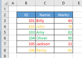
This article shows you how to format a row or column based on a cell value.
Let's take the example below of a worksheet containing three columns - ID, Name and Marks. You want to format each row based on Marks. If mark is more than 80 then the entire row will change the colour to green, between 50 and 80 will be in yellow and less than 50 in red.

Conditional formatting a row
- Select the cells that contain the data you want to format. In this example it is from cell B3 to D8.
- On Excel menu, click Home then from Styles group select Conditional Formatting → New Rule

- Select Use a formula to determine which cells to format.
- Enter the formula for the first rule.
=($D3 > 80 )

- Click Format then click Font tab and pick green colour and click Ok
- Click Ok again on the Formatting rule dialog.
- Repeat the above steps to create two more rules with the following formulas:
=($D3 < 50)   -- Set color to red.
=AND($D3>=50,$D3<80) -- set color to yellow.
- To edit or delete existing rules click Conditional Formatting → Manage Rules
Conditional formatting a column
Consider the example below where you have marks scored by pupils in vaarious subject and also their total marks. You want to automatically give a red color to column if the total marks is less than 250. This is how you do it.
=(C$7 < 250)
The procedure for conditionally formatting Rows and Columns are similar except for the formula. In case of column formatting, the dollar sign($) precedes the column reference in the formula (C$7 < 250) and in case of Row formatting, the $ sign is for the row reference ($D3 > 80 ).


