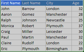
Quite often you'll come across excel sheets which contain duplicated and you may want to get rid of. You can have different interpretation for Here we show you how to remove, highlight or filter duplicate data in an Excel 2016 spreadsheet.
You can have different interpretations for duplicate data. For example you may have two identical rows of data like below:
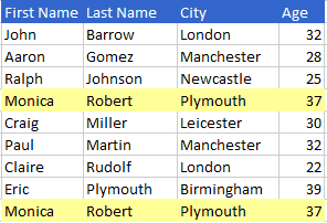
or same cell values in a single column
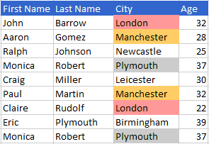
or same cell values in a range of cells
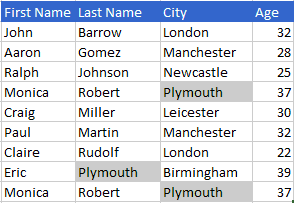
Removing duplicate rows
To remove (permanently delete) duplicate rows :
- Select the cell range you want to check. You may also select any header rows also.
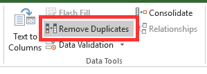
- Click the Data menu tab, then from Data Tools group click Remove Duplicates
- Select all the columns and check the box "My data has headers" if your selected range of data contains header rows.

- Click OK and a message box will tell you how many duplicate rows have been removed.

- The resulting data, after one row is removed will be like this
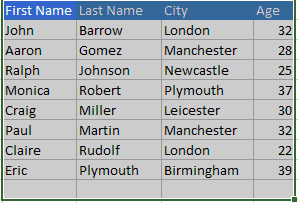
Remove duplicate cell values in a column
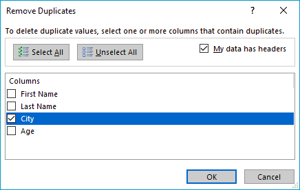
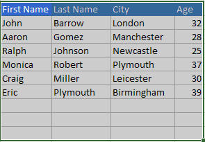
To remove duplicate cell values in a column or columns, the procedure is same as above except that you select only those specific columns you want to check. For example you select only the column City
The resulting sheet will be like this
Highlight duplicate values
Now, let's see how to highlight cells that contain duplicate value instead of deleting them.
- Select the cell range you want to check.
- Click Home then from Styles group select Conditional Formatting → Highlight Cell Rules → Duplicate Values
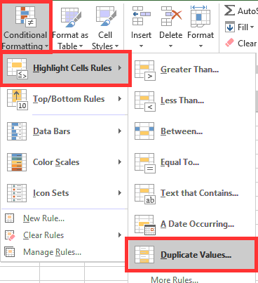
- Select Duplicate and a color scheme for highlighting, then click OK.

- Here is the result.

Filter duplicate rows
Another option for handling duplicate data is to hide or filter duplicate rows. This is how you do it.
- Select the cell range you want to check
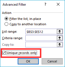
- Click Data from menu. From Sort & Filter group select Advanced

- Select the action Filter the list, in place and check the box next to Unique Records only. Click OK.
- Here is the result.
